NOTE & BLOG

When we navigate through the ocean of divide and conquer, there's a question that must be addressed—how is the time complexity of divide and conquer algorithms calculated?

From Divide and Conquer to Recurrence Relation

Divide and conquer involves breaking down a large problem into smaller subproblems and then merging the solutions of these subproblems to obtain the solution to the original problem. Recurrence relation is a mathematical way of modeling the time cost of this process.

Starting with a concrete example makes it easier to understand. Taking merge sort as an example, let $T(n)$ represent the time complexity of the original problem, where $n$ is the size of the input data. In the first split, the original data is divided into two equal parts, each of size $n/2$. Then, recursive calls to merge sort are made on these two parts, and the time complexity of this part is $2 T(n/2)$. Finally, the two sorted subarrays are merged, requiring a time complexity of $\Theta(n)$.

Based on the analysis above, we can write the recurrence relation for merge sort as follows:

$$\begin{equation} T(n) = \left\{ \begin{aligned} &\Theta(1) & \text{if } n=1\\ &2 T(n/2) + \Theta(n) & \text{if } n>1 \end{aligned} \right. \tag{1} \end{equation}$$

It can be imagined that for any divide and conquer algorithm, its time complexity can be expressed as a recurrence relation. The right-hand side of the recurrence relation usually consists of two parts: the total cost of the divided subproblems and the total cost of dividing and merging subproblems. The first part remains a function of $T$, while the second part represents the actual asymptotic complexity.

Having a recurrence relation is not sufficient to determine the exact time complexity of the algorithm. We need to further calculate the actual solution $T(n)$.

Substitution Method

The first method for solving recurrence relations is called the substitution method. We need to guess the form of the solution first and then use mathematical induction to prove that the guess is correct.

For Equation (1), let's assume that our guess for the solution is $T(n) = O(n \log n)$. If we remove the asymptotic notation, this equation is equivalent to $T(n) \le c_1 n \log n$, where $c_1$ is any positive constant.

According to mathematical induction, we first need to establish that the guess holds for small values of $n$. When $n=1$, according to Equation (1), $T(1) = \Theta(1) = d_1$, where $d_1$ is some constant greater than 0. According to the guess, we hope $T(1) \le c_1 \log 1 = 0$, but no matter how we choose $c_1$, this equation cannot hold because $T(1) = d_1$ is always greater than 0. The mathematical induction fails before it even starts.

However, there is no need to worry; this is just a special case caused by $\log 1 = 0$. We can place the initial state of mathematical induction at $n>1$ without affecting the results of mathematical induction. We are only interested in the asymptotic properties of $T(n)$ when $n$ is sufficiently large, not in the initial stage.

Now, let $n = 2$, then $T(2) = 2T(1) + d_2 = 2d_1 + d_2$. We hope that $T(2) \le c_1 \log 2$ holds. Simplifying, we get $c_1 \ge d_1 + d_2/2$. Since $d_1$ and $d_2$ are constants, such $c_1$ exists, and the initial condition holds.

Next, mathematical induction assumes that the solution holds at $n/2$, i.e., $T(n/2) \le c_1 \frac{n}{2} \log\frac{n}{2} = \frac{1}{2}c_1n(\log n - 1)$. Then we prove that $T(n) \le c_1 n \log n$ also holds.

Substituting $T(n/2)$ into Equation (1), we get

$$\begin{equation} \begin{aligned} T(n) & = 2 T\left(\frac{n}{2}\right) + \Theta(n) \\ & \le 2 \frac{1}{2}c_1n(\log n - 1) + d_2n \\ & = c_1 n \log n + (d_2 - c_1) n \\ & \le c_1 n \log n \end{aligned} \end{equation}$$

Where the last line's inequality requires $d_2 - c_1 < 0$, obviously such $c_1$ exists, so the proof is complete.

Thus, we have proved that $T(n) = O(n \log n)$ is the solution to the recurrence relation (1). However, this is not the end; this asymptotic notation is not a tight bound. Can we further guess that $T(n) = \Theta(n \log n)$ holds? This is indeed a good idea. So, as we proceed, as long as we can prove that $T(n) = \Omega(n \log n)$ holds, we can obtain the tight bound mentioned above. Removing the asymptotic notation, this equation is equivalent to $T(n) \ge c_2 n \log n$. Using mathematical induction again, confirming that this holds in the initial stage, and then assuming that the solution holds at $n/2$, we can derive that the solution holds at $n$. Therefore, the proof is complete. Since the proof steps are almost identical to those just mentioned, we will not elaborate on them, and you can try it yourself.

The substitution method relies on accurate guesses, which can be impractical. Therefore, in practice, a more common approach is to find a guess using other methods and then use the substitution method to verify the guess. The recursive tree method we will introduce next provides this possibility.

Recursive Tree

Expanding the recurrence relation layer by layer directly yields a tree structure. For example, let's take $T(n) = 3 T(n/4) + \Theta(n^2)$ as an example and see how to draw its recursive tree.

Expanding the first layer, we draw three child nodes under the root node.

Here, $cn^2$ represents the cost of decomposition and merging at this layer, which corresponds to the part represented by $\Theta(n^2)$ in the recurrence relation.

Next, further expand to the second layer.

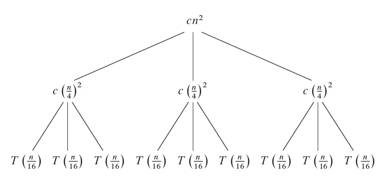
Here, the cost of each node in the first layer is still $c(\frac{n}{4})^2$, still corresponding to the part represented by $\Theta(n^2)$ in the recurrence relation, but the data size has changed from $n$ to $n/4$.

Continue expanding in this way until the leaf nodes.

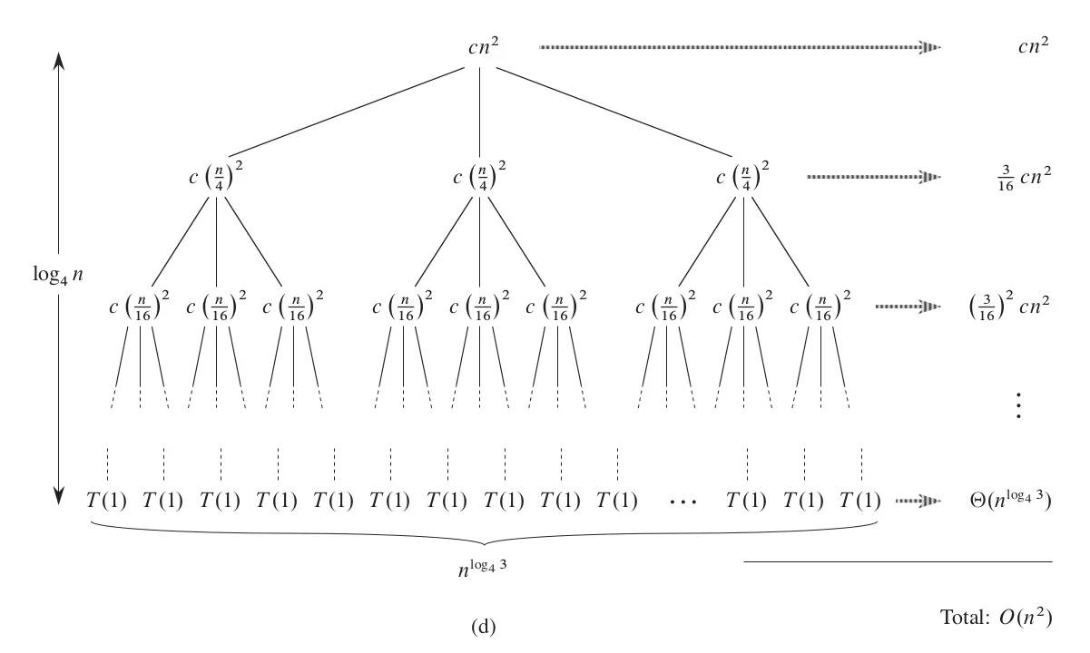
This completes a complete recursive tree. The data size of each layer is reduced to one-fourth of the previous one, until the data size of the leaf node is 1, so the total number of layers is $\log_4 n$. The rightmost side of the figure calculates the total cost of all nodes in each layer, and the calculation is simple: multiply the cost of a single node by the number of nodes in that layer. In the last layer, the cost of a single node is a constant, and the number of nodes is $3^{\log_4 n} = n^{\log_4 3}$, and we denote the total cost as $\Theta(n^{\log_4 3})$.

Next, we just need to add up the costs of all nodes to obtain the solution to the recurrence relation.

$$\begin{aligned} T(n) &= cn^2 + \frac{3}{16} cn^2 + \left(\frac{3}{16}\right)^2 cn^2 + \cdots + \left( \frac{3}{16} \right)^{\log_4 n-1} cn^2 + \Theta(n^{\log_4 3}) \\ &=\sum_{i=0}^{\log_4 n-1}{\left(\frac{3}{16}\right)^i cn^2} + \Theta(n^{\log_4 3})\\ &\lt \sum_{i=0}^{\infty}{\left(\frac{3}{16}\right)^i cn^2} + \Theta(n^{\log_4 3}) \\ &= \frac{1}{1 - 3/16}cn^2 + \Theta(n^{\log_4 3}) \\ &= \frac{16}{13} cn^2 + \Theta(n^{\log_4 3}) \\ &= O(n^2) \end{aligned}$$

Here, in the third line, we made a simplification by replacing a finite geometric series with an infinite geometric series. Although the total size has increased, this infinite decreasing geometric series has a limit, so this replacement can simplify the derivation process. The second term in the fifth line is a lower-order term relative to the first term, so it is discarded, resulting in the final result.

Similar to before, we have only proven the upper bound of the recurrence relation. Naturally, we want to try whether it can also be proven as a lower bound. In the above equation, each term in the summation contains $cn^2$, and each term is positive, so $T(n) = \Omega(n^2)$ obviously holds. Therefore, the solution to the recurrence relation is $T(n) = \Theta(n^2)$.

In this example, we directly calculated the solution to the recurrence relation using the recursive tree method. Of course, we can use the substitution method to verify whether this solution is correct. In some cases, it may be slightly difficult to calculate the exact solution using the recursive tree method, but it does not prevent us from making a reasonable guess and then further verifying this guess using the substitution method.

Master Theorem

Both the substitution method and the recursion tree method have their drawbacks. The former requires an accurate guess, while the latter involves drawing a recursion tree and deriving results. If you derive too much, you may find that the forms of most recursive solutions seem to be the same. From the derivation process above, it can be observed that the final solution depends entirely on the sum of costs in the middle layers and has nothing to do with the leaf layer because the latter is a lower-order term. In other recursion trees, the final solution may depend entirely on the cost of the leaf layer, unrelated to the middle layers. Therefore, we may be able to classify recursive formulas and directly write out the final solution according to some rules. This is the idea behind the master theorem.

When the divide-and-conquer method evenly splits the data each time, the recursive formula generally has the following form.

$$T(n) = aT\left(\frac{n}{b}\right) + f(n) \tag{2}$$

where $a$ is a positive integer representing the number of subproblems when dividing each time, $b$ is an integer greater than 1 representing the reduction factor in problem size each time, and $f(n)$ is an asymptotically positive function representing the cost of dividing and merging.

To find a unified solution applicable to any $a$, $b$, and $f(n)$, we still need to use the recursion tree to calculate the costs of all intermediate and leaf nodes and try to derive a simple result.

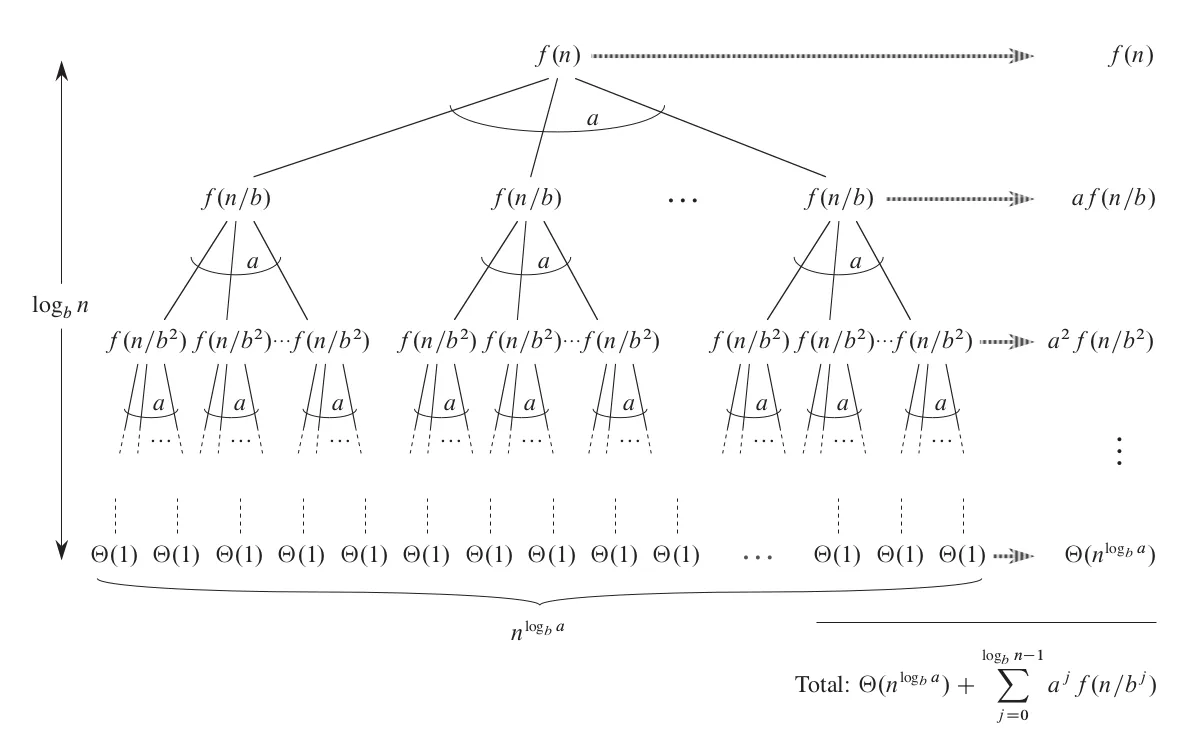
From the graph, we can see that the total cost of all nodes is $T(n) = \Theta(n^{\log_b a}) + \sum_{j=0}^{\log_b n-1}{a^j f(n/b^j)}$. Further derivation requires a breakthrough idea, and I don't know how the original researchers discovered the following pattern, but it is indeed magical.

Researchers found that the relationship between $f(n)$ and $\Theta(n^{\log_b a})$ determines the final simplified form of $\sum_{j=0}^{\log_b n-1}{a^j f(n/b^j)}$. Define

$$g(n) = \sum_{j=0}^{\log_b n-1}{a^j f(n/b^j)} \tag{3}$$

Now let's analyze three cases.

1. If $\Theta(n^{\log_b a})$ is larger, we can assume that there exists a constant $\epsilon > 0$ such that $f(n) = O(n^{\log_b a-\epsilon})$. Substituting this into the summation formula, it can be simplified to $g(n) = O(n^{\log_b a})$.

2. If both are equally large, directly substitute into equation (3) and simplify to get $g(n) = \Theta(n^{\log_b a} \log n)$.

3. If $f(n)$ is larger and, for some constant $c < 1$, for all sufficiently large $n$, $a f(n/b) \le c f(n)$ holds, then it can be deduced that $g(n) = \Theta(f(n))$.

Here, the complete proof process is not provided, partly because I don't want to make it too long, and secondly, I feel that these proofs are somewhat cumbersome and not very meaningful. Interested students can refer to the original book.

Substituting the functions $g(n)$ for these three cases into the complete solution, we get:

• For case 1: $T(n) = \Theta(n^{\log_b a}) + O(n^{\log_b a}) = \Theta(n^{\log_b a})$

• For case 2: $T(n) = \Theta(n^{\log_b a}) + \Theta(n^{\log_b a} \log n) = \Theta(n^{\log_b a} \log n)$

• For case 3: $T(n) = \Theta(n^{\log_b a}) + \Theta(f(n)) = \Theta(f(n))$

Now, for any recursive formula, we only need to determine which case it belongs to and directly substitute into the corresponding formula. To facilitate understanding, let's go through a few examples.

Example 1:

$T(n) = 9 T(n/3) + n$

For this recursive formula, we have $a = 9$, $b = 3$, $f(n) = n$. Since $f(n) = n$ is asymptotically smaller than $\Theta(n^2)$, it can be applied to the first case of the master theorem, and the solution is $T(n) = \Theta(n^2)$.

Example 2:

$T(n) = T(2n/3) + 1$

For this formula, $a = 1$, $b = 3/2$, $f(n) = 1$. Since $n^{\log_b a} = n^{\log_{3/2} 1} = n^0 = 1$, which is exactly equal to $f(n)$, it can be applied to the second case of the master theorem, and the solution is $T(n) = \Theta(\log n)$.

Example 3:

$T(n) = 3T(n/4) + n\log n$

For this formula, $a = 3$, $b = 4$, $f(n) = n\log n$. Since $n^{\log_b a} = n^{\log_4 3} = n^{0.793}$, and $f(n) = n\log n$ is asymptotically larger than $n^{0.793}$, it should consider the third case of the master theorem. However, we need to check if the additional condition holds: for some constant $c < 1$ and all sufficiently large $n$, $a f(n/b) \le c f(n)$ holds. Substituting $a$, $b$, and $f(n)$ into the inequality, we get

$$3\frac{n}{4}\log\frac{n}{4} \le cn\log n \implies \frac{3}{4}( \log n - 2) \le c\log n \implies \left(\frac{3}{4} - c\right) \log n \le \frac{3}{2}$$

When $c \ge \frac{3}{4}$, this inequality always holds, and the additional condition is satisfied. Therefore, it can be applied to the third case of the master theorem, and the solution is $T(n) = \Theta(n\log n)$.

Example 4:

$T(n) = 2T(n/2) + n\log n$

For this formula, $a = 2$, $b = 2$, $f(n) = n\log n$. Since $n^{\log_b a} = n^{\log_2 2} = n$, and $f(n) = n\log n$ is asymptotically larger than $n$, it should consider the third case of the master theorem. Substituting $a$, $b$, and $f(n)$ into the inequality, we get

$$2\frac{n}{2}\log\frac{n}{2} \le cn\log n \implies \log n - 1 \le c\log n \implies (1-c)\log n \le 1$$

When $c \ge 1$, this inequality always holds. However, the additional condition requires $c < 1$, so this case cannot be applied to the third case of the master theorem. In other words, not all recursive formulas of the form $T(n) = a T(n/b) + f(n)$ can be solved using the master theorem; there is a gap between cases two and three. In such cases, we can only use the recursion tree method. Students can try it, and the result will be $T(n) = \Theta(n \log^2 n)$.

After going through these four examples, have you mastered the master theorem? If you have any questions, please leave a comment, and I will reply as soon as possible.

The study of algorithms is endless, and the calculation of time complexity is fundamental and should not be underestimated.

Details

Careful readers may notice that in the fourth case mentioned above, although $nlgn$ grows asymptotically faster than $n$, it is not asymptotically greater in the polynomial sense because there is no $\epsilon > 0$ such that $nlgn = \Omega \left( n^{1+\epsilon} \right)$ holds. On the contrary, $nlgn = o \left( n^{1+\epsilon} \right)$ holds for any $\epsilon > 0$. So, in fact, this case does not need to be judged for regular conditions to draw conclusions in advance. However, in the third case in the previous text, I did not emphasize asymptotic greater in the polynomial sense, not because I forgot to write it, but because this condition is not needed at all.

For any recurrence relation that fits the master theorem format, if it satisfies the regular conditions in case three, then it must satisfy $f\left(n\right) = \Omega \left( n^{log_b a + \epsilon} \right)$." The specific proof details can be found in this answer on StackExchange, and are not detailed here.

Although regular conditions can imply $f\left(n\right) = \Omega \left( n^{log_b a + \epsilon} \right)$, the reverse is not true. We can construct the following function:

$T\left(n\right) = T\left(n/2\right) + n\left( 2 - \cos n \right)$

Here, $a=1$, $b=2$, and $f\left(n\right) = n \left( 2 - \cos n \right) = \Omega \left( n^{log_2 1+ \epsilon} \right) = \Omega \left( n^\epsilon \right)$ holds for any $\epsilon \le1$. However, when applying the regular condition:

$\begin{aligned} f\left(n / 2\right) &\le c f\left(n\right) \\ \frac{n}{2} \left(2 - \cos \frac{n}{2} \right) & \le c \left( 2 - \cos n \right) \end{aligned}$

For any $c \lt 1$, the right side must be $c \left( 2 - \cos n \right) \lt 3$. However, the left side, when $n$ is large enough, must be greater than $3$. Therefore, this equation cannot hold, and the regular condition is not satisfied.

Reference

These cases are from the Wikipedia entry on Master theorem.